Supervised ML workflow for building forecasting models on univariate time series data.
Uses the seaice dataset from seaborn, and applies several time series models to forecast sea ice extent (Naive Mean, ARIMA, Exponential Smoothing, LightGBM with lagged features, Theta).
This dataset contains no missing values, so no imputation is used.
This script does the following:
Splits the data into train and test sets
Scales data before training (except for AutoARIMA and ExponentialSmoothing, which typically work with unscaled data)
Trains each model on the training set and evaluates on test set.
Plots the full series for visual inspection of model performance
Note: Using display for HTML tables
print(summarize(df)) and print(df.head()) return tables printed in plain text. To get nicer-formatted HTML tables, use the following instead of print():
from IPython.display import displaydisplay(df.head())# Display summarydisplay(summarize(df))
Import and Check Data
import warningsimport timeimport numpy as npimport pandas as pdimport seaborn as snsimport matplotlib.pyplot as pltfrom minieda import summarize # pip install git+https://github.com/dbolotov/minieda.gitfrom darts import TimeSeriesfrom darts.models import NaiveMean, AutoARIMA, ExponentialSmoothing, LightGBMModel, Thetafrom darts.dataprocessing.transformers import Scalerfrom darts.utils.utils import ModelMode, SeasonalityModefrom darts.metrics import mae, rmsefrom sklearn.linear_model import LinearRegression# Suppress sklearn warningswarnings.filterwarnings("ignore", category=UserWarning, module="sklearn")# Display and plot settingspd.set_option("display.width", 220)plt.rcParams.update({'font.size': 9})# Load dataset and display first few rowsdf = sns.load_dataset("seaice")print("\n----- First Few Rows of Data -----\n")print(df.head())# Display summaryprint("\n----- Data Summary -----\n")print(summarize(df, include_perc=False, sort=True))
----- First Few Rows of Data -----

        Date  Extent
0 1980-01-01  14.200
1 1980-01-03  14.302
2 1980-01-05  14.414
3 1980-01-07  14.518
4 1980-01-09  14.594

----- Data Summary -----

                 dtype  count  unique  missing  zero   mean   std   min    50%    max  skew
Extent         float64  13175    7649        0     0  11.29  3.28  3.34  11.98  16.41 -0.44
Date    datetime64[ns]  13175   13175        0     0
Transform Data
# Sort by date and set Date as indexdf = df.sort_values("Date").set_index("Date")# Resample to different frequency using linear interpolationdf_resampled = df.resample("MS").interpolate("linear") # monthly# Drop any missing values (usually at the edges)df_resampled = df_resampled.dropna()# Convert to Darts TimeSeries, allowing it to infer frequencydts = TimeSeries.from_series(df_resampled["Extent"], fill_missing_dates=True, freq=None)# Show darts infoprint("\n----- darts TimeSeries Summary -----\n")print("frequency: ", dts.freq_str)# Split the series into training and test setstest_frac =0.15n_test =int(len(dts) * test_frac)train, test = dts[:-n_test], dts[-n_test:]# Confirm split sizesprint(f"Train range: {train.start_time().date()} to {train.end_time().date()} ({train.n_timesteps} steps)")print(f"Test range: {test.start_time().date()} to {test.end_time().date()} ({test.n_timesteps} steps)")# Normalizescaler = Scaler()train_scaled = scaler.fit_transform(train)test_scaled = scaler.transform(test)
----- darts TimeSeries Summary -----

frequency:  MS
Train range: 1980-01-01 to 2013-12-01 (408 steps)
Test  range: 2014-01-01 to 2019-12-01 (72 steps)
Train Models
# Initialize modelsmodels = {"NaiveMean": NaiveMean(),"AutoARIMA": AutoARIMA(season_length=12, max_p=2, max_q=2, max_P=1, max_Q=1, max_d=1, max_D=1),"ExponentialSmoothing": ExponentialSmoothing(trend=ModelMode.ADDITIVE, seasonal=SeasonalityMode.ADDITIVE, seasonal_periods=12,damped=True),"LightGBMModel": LightGBMModel(lags=12, output_chunk_length=1, random_state=42, verbose=-1, force_col_wise=True),"Theta": Theta(season_mode=SeasonalityMode.ADDITIVE),}# ---- TRAIN MODELS AND PREDICT ----results = []forecasts_test = {}print("\n----- Training Models -----\n")for name, model in models.items():print(f"Training {name}...") start_time = time.time()# Use unscaled data for ARIMA and ExponentialSmoothingif name in ["AutoARIMA", "ExponentialSmoothing"]: model.fit(train) pred_test = model.predict(n=len(test))else: model.fit(train_scaled) pred_test_scaled = model.predict(n=len(test_scaled)) pred_test = scaler.inverse_transform(pred_test_scaled) train_duration = time.time() - start_time forecasts_test[name] = pred_test# Evaluate on test set results.append({"Model": name,"MAE": mae(test, pred_test),"RMSE": rmse(test, pred_test),"Train Time (s)": train_duration })
----- Training Models -----

Training NaiveMean...
Training AutoARIMA...
Training ExponentialSmoothing...
Training LightGBMModel...
Training Theta...
Evaluate and Plot Forecasts
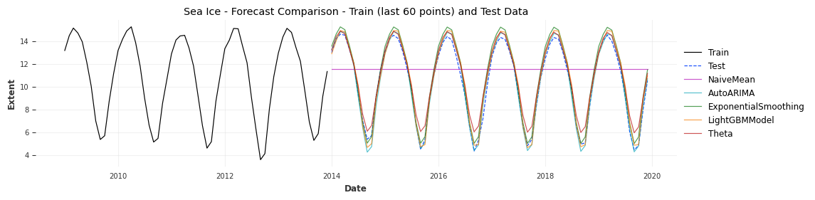
# Display resultsresults_df = pd.DataFrame(results).sort_values("RMSE")print(results_df.to_string(index=False))# Plot: final 60 train + full test + predictions on testtrain_to_plot = train[-60:] # last 60 points from trainplt.figure(figsize=(12, 3))# Plot actual datatrain_to_plot.plot(label="Train", linewidth=0.9)test.plot(label="Test", linewidth=0.9, alpha=0.9, linestyle="--")# Plot forecasts made on test setfor name, forecast in forecasts_test.items():if forecast isnotNone: forecast.plot(label=name, linewidth=0.9, alpha=0.7)plt.title("Sea Ice - Forecast Comparison - Train (last 60 points) and Test Data")plt.xlabel("Date")plt.ylabel("Extent")plt.legend(loc="center left", bbox_to_anchor=(1.0, 0.5))plt.grid(True, alpha=0.4)plt.tight_layout()plt.show()
               Model      MAE     RMSE  Train Time (s)
           AutoARIMA 0.325538 0.411305        2.387773
       LightGBMModel 0.438801 0.531785        0.127118
ExponentialSmoothing 0.577775 0.667614        0.113169
               Theta 0.605557 0.756212        0.006058
           NaiveMean 2.937516 3.581656        0.000978