Supervised ML workflow for building a regression model on tabular data with categorical and continuous features.
Uses the tips dataset from seaborn, and trains several models to predict the tip amount. Uses scikit-learn for pre-processing, modeling, and evaluation.
This dataset contains no missing values, so imputation is not used.
This script:
Includes train/test split
Handles categorical and numerical features separately
Runs a grid search to find best model parameters for several models: linear regression, lasso, ridge, random forest regressor, knn regressor, xgboost regressor
Evaluates results using RMSE, MAE, R² score
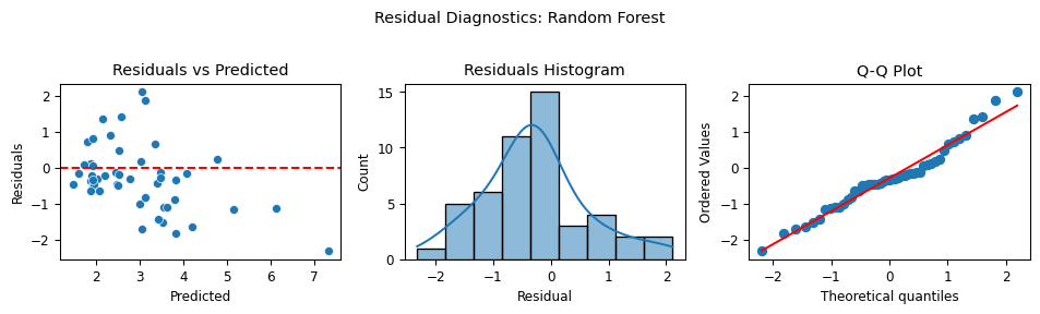
Creates 3 plots for evaluating residuals per model
Predicts target on a fictional example
Note: Using display for HTML tables
print(summarize(df)) and print(df.head()) return tables printed in plain text. To get nicer-formatted HTML tables, use the following instead of print():
from IPython.display import displaydisplay(df.head())# Display summarydisplay(summarize(df))
import seaborn as snsimport pandas as pdfrom minieda import summarize # pip install git+https://github.com/dbolotov/minieda.gitimport timefrom pprint import pprintfrom sklearn.linear_model import LinearRegression, Lasso, Ridgefrom sklearn.ensemble import RandomForestRegressorfrom sklearn.neighbors import KNeighborsRegressorfrom xgboost import XGBRegressorfrom sklearn.model_selection import train_test_splitfrom sklearn.compose import ColumnTransformerfrom sklearn.preprocessing import OneHotEncoder, StandardScalerfrom sklearn.pipeline import Pipelinefrom sklearn.model_selection import GridSearchCVfrom sklearn.metrics import root_mean_squared_error, mean_absolute_error, r2_scorefrom scipy import statsimport matplotlib.pyplot as pltplt.rcParams.update({'font.size': 9}) # set global plot paramspd.set_option("display.width", 220) # set display width for printed tables# Load dataset and display first few rowsdf = sns.load_dataset("tips")print("----- SCRIPT OUTPUT -----")print("\n----- First Few Rows of Data -----\n")print(df.head())# Display summaryprint("\n----- Data Summary -----\n")print(summarize(df))# Define columnscat_cols = ['sex', 'smoker', 'day', 'time']num_cols = ['total_bill', 'size']# Split the dataX = df[cat_cols + num_cols]y = df['tip']# Split into training and testX_train, X_test, y_train, y_test = train_test_split( X, y, test_size=0.2, random_state=42)# Define preprocessing for numeric and categorical featuresnumeric_preprocessing = Pipeline([ ('scale', StandardScaler())])categorical_preprocessing = Pipeline([ ('encode', OneHotEncoder(drop='first', sparse_output=False)) # one-hot; drop first feature to avoid multicollinearity])# Combine into a column transformerpreprocessor = ColumnTransformer([ ('num', numeric_preprocessing, num_cols), ('cat', categorical_preprocessing, cat_cols)])# Define models and hyperparameters to optimizemodels = [ {"name": "LinearRegression","estimator": LinearRegression(),"param_grid": None }, {"name": "Ridge","estimator": Ridge(),"param_grid": {"model__alpha": [0.1, 1.0, 10.0] } }, {"name": "Lasso","estimator": Lasso(),"param_grid": {"model__alpha": [0.1, 1.0, 10.0] } }, {"name": "RandomForest","estimator": RandomForestRegressor(random_state=42),"param_grid": {"model__n_estimators": [20,30],"model__max_depth": [None, 10],"model__min_samples_split": [2, 5] } }, {"name": "KNN","estimator": KNeighborsRegressor(),"param_grid": {"model__n_neighbors": [3, 5, 7] } }, {"name": "XGBoost","estimator": XGBRegressor(random_state=42, verbosity=0),"param_grid": {"model__n_estimators": [30, 50],"model__learning_rate": [0.1, 0.3],"model__max_depth": [3, 6] } }]results = []print("\n----- GRID SEARCH WITH BEST RESULT ON TRAIN AND TEST SETS -----")start_time = time.time()trained_models = {}for m in models:print(f"\n--- {m['name']} ---") pipeline = Pipeline([('pre', preprocessor), ('model', m["estimator"])])if m["param_grid"]: search = GridSearchCV( pipeline, m["param_grid"], scoring="neg_root_mean_squared_error", # RMSE cv=3, n_jobs=-1, verbose=1 ) search.fit(X_train, y_train) best_model = search.best_estimator_print("Best params:", search.best_params_)else: #if no parameters to optimize pipeline.fit(X_train, y_train) best_model = pipeline trained_models[m["name"]] = best_model# Predict and evaluate on both train and test y_train_pred = best_model.predict(X_train) y_test_pred = best_model.predict(X_test) train_rmse = root_mean_squared_error(y_train, y_train_pred) test_rmse = root_mean_squared_error(y_test, y_test_pred) train_mae = mean_absolute_error(y_train, y_train_pred) test_mae = mean_absolute_error(y_test, y_test_pred) train_r2 = r2_score(y_train, y_train_pred) test_r2 = r2_score(y_test, y_test_pred)print("")print(f"{'Metric':<6} | {'Train':>6} | {'Test':>6}")# print("-" * 24)print(f"{'RMSE':<6} | {train_rmse:>6.4f} | {test_rmse:>6.4f}")print(f"{'MAE':<6} | {train_mae:>6.4f} | {test_mae:>6.4f}")print(f"{'R²':<6} | {train_r2:>6.4f} | {test_r2:>6.4f}")# results.append({# "model": m["name"],# "rmse": rmse,# "mae": mae,# "r2": r2# }) results.append({"model": m["name"],"train_rmse": train_rmse,"test_rmse": test_rmse,"train_mae": train_mae,"test_mae": test_mae,"train_r2": train_r2,"test_r2": test_r2 })print(f"\nGrid search completed in {time.time() - start_time:.2f} seconds")print("\n----- EVALUATION SUMMARY -----\n")print(pd.DataFrame(results).sort_values("test_rmse", ascending=False))print("\n")def plot_residual_diagnostics(y_true, y_pred, model_name="Model"): residuals = y_true - y_pred fig, axes = plt.subplots(1, 3, figsize=(10, 3)) fig.suptitle(f"Residual Diagnostics: {model_name}")# 1. Residuals vs Predicted sns.scatterplot(x=y_pred, y=residuals, ax=axes[0]) axes[0].axhline(0, color="red", linestyle="--") axes[0].set_xlabel("Predicted") axes[0].set_ylabel("Residuals") axes[0].set_title("Residuals vs Predicted")# 2. Histogram of residuals sns.histplot(residuals, kde=True, ax=axes[1]) axes[1].set_title("Residuals Histogram") axes[1].set_xlabel("Residual")# 3. Q-Q Plot stats.probplot(residuals, dist="norm", plot=axes[2]) axes[2].set_title("Q-Q Plot") axes[2].get_lines()[0].set_color("tab:blue") # points axes[2].get_lines()[1].set_color("red") # reference line plt.tight_layout(rect=[0, 0, 1, 0.95]) plt.show()y_test_pred = trained_models["RandomForest"].predict(X_test)plot_residual_diagnostics(y_test, y_test_pred, model_name="Random Forest")# Predict on a new examplenew_sample = pd.DataFrame([{'sex': 'Female','smoker': 'No','day': 'Sun','time': 'Dinner','total_bill': 40.0,'size': 2}])# Predict on fictional sample with each modelpredictions = []for model_name, model in trained_models.items(): pred = model.predict(new_sample)[0] predictions.append({"model": model_name, "predicted_tip": round(pred, 2)})# Display predictionsprint("----- PREDICTIONS ON NEW SAMPLE -----")print("\n----- Sample Input -----")print(new_sample)print("\n----- Sample Predictions -----\n")print(pd.DataFrame(predictions).sort_values("predicted_tip", ascending=False))
----- SCRIPT OUTPUT -----

----- First Few Rows of Data -----

   total_bill   tip     sex smoker  day    time  size
0       16.99  1.01  Female     No  Sun  Dinner     2
1       10.34  1.66    Male     No  Sun  Dinner     3
2       21.01  3.50    Male     No  Sun  Dinner     3
3       23.68  3.31    Male     No  Sun  Dinner     2
4       24.59  3.61  Female     No  Sun  Dinner     4

----- Data Summary -----

               dtype  count  unique  unique_perc  missing  missing_perc  zero  zero_perc     top freq   mean   std   min   50%    max  skew
total_bill   float64    244     229        93.85        0           0.0     0        0.0               19.79   8.9  3.07  17.8  50.81  1.13
tip          float64    244     123        50.41        0           0.0     0        0.0                 3.0  1.38   1.0   2.9   10.0  1.47
size           int64    244       6         2.46        0           0.0     0        0.0                2.57  0.95   1.0   2.0    6.0  1.45
sex         category    244       2         0.82        0           0.0     0        0.0    Male  157
smoker      category    244       2         0.82        0           0.0     0        0.0      No  151
day         category    244       4         1.64        0           0.0     0        0.0     Sat   87
time        category    244       2         0.82        0           0.0     0        0.0  Dinner  176

----- GRID SEARCH WITH BEST RESULT ON TRAIN AND TEST SETS -----

--- LinearRegression ---

Metric |  Train |   Test
RMSE   | 1.0491 | 0.8387
MAE    | 0.7600 | 0.6671
R²     | 0.4582 | 0.4373

--- Ridge ---
Fitting 3 folds for each of 3 candidates, totalling 9 fits
Best params: {'model__alpha': 10.0}

Metric |  Train |   Test
RMSE   | 1.0507 | 0.8283
MAE    | 0.7623 | 0.6657
R²     | 0.4567 | 0.4511

--- Lasso ---
Fitting 3 folds for each of 3 candidates, totalling 9 fits
Best params: {'model__alpha': 0.1}

Metric |  Train |   Test
RMSE   | 1.0615 | 0.7824
MAE    | 0.7777 | 0.6548
R²     | 0.4454 | 0.5102

--- RandomForest ---
Fitting 3 folds for each of 8 candidates, totalling 24 fits
Best params: {'model__max_depth': 10, 'model__min_samples_split': 2, 'model__n_estimators': 30}

Metric |  Train |   Test
RMSE   | 0.4436 | 0.9459
MAE    | 0.3313 | 0.7394
R²     | 0.9032 | 0.2842

--- KNN ---
Fitting 3 folds for each of 3 candidates, totalling 9 fits
Best params: {'model__n_neighbors': 5}

Metric |  Train |   Test
RMSE   | 0.9195 | 0.9025
MAE    | 0.6846 | 0.7160
R²     | 0.5839 | 0.3484

--- XGBoost ---
Fitting 3 folds for each of 8 candidates, totalling 24 fits
Best params: {'model__learning_rate': 0.1, 'model__max_depth': 3, 'model__n_estimators': 30}

Metric |  Train |   Test
RMSE   | 0.7910 | 0.8755
MAE    | 0.5830 | 0.7102
R²     | 0.6920 | 0.3868

Grid search completed in 2.76 seconds

----- EVALUATION SUMMARY -----

              model  train_rmse  test_rmse  train_mae  test_mae  train_r2   test_r2
3      RandomForest    0.443583   0.945898   0.331275  0.739375  0.903152  0.284205
4               KNN    0.919482   0.902499   0.684636  0.716000  0.583873  0.348381
5           XGBoost    0.791011   0.875502   0.583020  0.710206  0.692033  0.386783
0  LinearRegression    1.049133   0.838664   0.759965  0.667133  0.458249  0.437302
1             Ridge    1.050658   0.828321   0.762260  0.665704  0.456673  0.451095
2             Lasso    1.061543   0.782438   0.777739  0.654809  0.445356  0.510221


----- PREDICTIONS ON NEW SAMPLE -----

----- Sample Input -----
      sex smoker  day    time  total_bill  size
0  Female     No  Sun  Dinner        40.0     2

----- Sample Predictions -----

              model  predicted_tip
0  LinearRegression           4.93
3      RandomForest           4.78
1             Ridge           4.77
2             Lasso           4.63
5           XGBoost           4.39
4               KNN           3.50